MR Methods Development
Developing new MR hardware and methods requires dedication, innovation, and a lot of debugging. Field monitoring gives you a direct view of your scanner's performance to reduce guesswork and frustration in finding those bugs.
Whether you are characterizing new hardware or trying to understand the errant performance of a new pulse sequence, there are many requirements to juggle and many possible frustration points. Field monitoring of the magnetic environment provides a direct, meaningful measurement of gradient hardware performance, gradient waveform and timing in pulse sequence development, and spatiotemporal phase accrual. This allows you to more quickly identify bugs, characterize new systems, and create the next generation of MR methods.
Standard methods of programming MR sequences can be a bit cumbersome. The vendors often provide sequence simulation tools, but they can either be error prone and unstable, or not reflect the physical environment of the scanner. Especially for demanding MR sequence tasks, such as diffusion or steady-state sequences, the difference between the programmed gradient waveform and the applied encoding field can make the difference between a coherent, geometrically precise signal and a signal corrupted by gradient timing errors or unfaithful gradient waveforms. The image below illustrates how a gradient trace which looks “OK” can belie undesired accruing phase. This is especially problematic for steady-state sequences, as breaking this steady-state assumption will invariably cause artefacts in the resulting images.
Fischer et al. understood that steady-state MR sequences can be sensitive to encoding field non-idealities. Balanced steady-state free precession (bSSFP) sequences have the advantage that under proper excitation, the signal of from each voxel reaches a ‘steady-state’ which is advantageous for acquisition in areas of high field inhomogeneity or when motion is present. bSSFP sequences require gradients to be stable and to not induce time varying fluctuations in the imaged sample. Any deviation from this condition results in easily observable banding artifacts. Phase encoding commonly breaks this condition and requires optimal ordering to reduce banding. They measured multiple phase encoding schemes and showed that accounting for nuisance phase reduced image artifacts.
In a similar way, the Radial k-space trajectory has a variety of systematic challenges. Below, you can see a radial acquisition, with time order indicated by coloration. Looking at the k-space trajectory overall, it looks fairly well characterized. Zooming in however to the center of k-space, where much of the image signal lies, we can see these imaging trajectories cross “0” at several different locations. Again, dismissing these sampling inaccuracies can cause artefacts in the reconstructed image!
Characterize gradients and resistive shims to improve waveform pre-emphasis
Dr. Vannesjo and the team at ETH utilized the Dynamic Field Camera during their development of a dynamic shim scheme which would optimize the shims for each slice of the image, improving the shims for hard to shim areas such as the orbits which are often poorly shimmed when considered with the rest of the head. Direct measurements of their shim system showed that the shims required several seconds to settle. Using the Dynamic Field Camera to measure shim dynamics, they developed a pre-emphasis scheme was effectively applied to dynamically switch their shim coils, enabling the dynamic shimming method.
Characterize custom gradient sets
Wilm et al. utilized a recently designed high slew rate (up to 1200 T/m/s), head only gradient set to develop fast spiral imaging (see also Hennel, et al.). The high slew rate gradient set allows k-space to be traversed more quickly during the imaging readout, allowing one to sample all of the relevant portions of acquisition space before the signal has decayed away. The gradient system is asymmetric and as such, concomitant fields were expected. Characterizing fields in specialty gradient sets such as this one is important for generating appropriate reconstructions and pre-emphasis schemes.
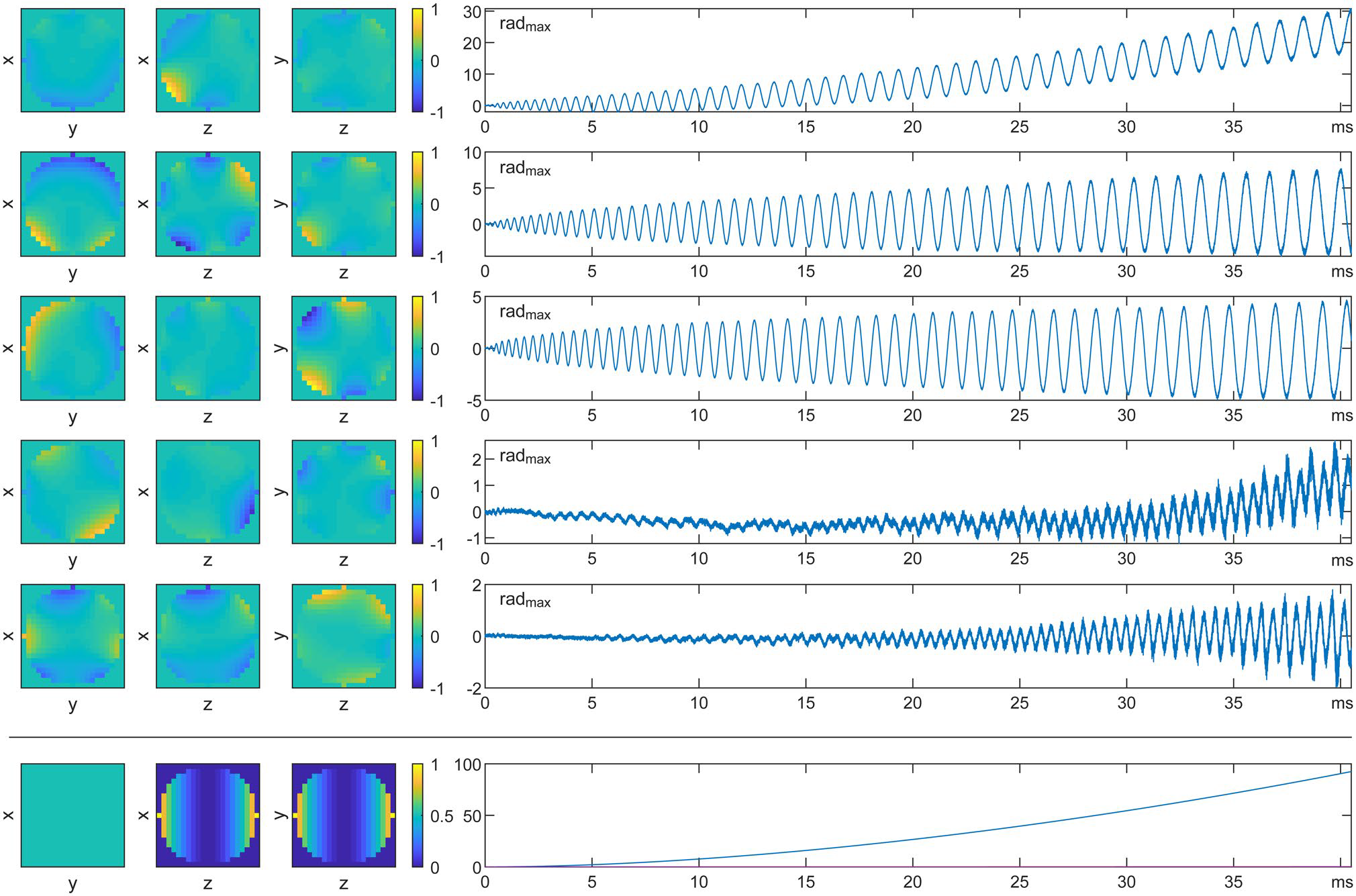
These results are also impactful in that they calculated the acquired k-space traversal up to 5th order spherical harmonics. They generated a dataset capable of fitting 5th order spherical harmonics by combining multiple datasets from the Dynamic Field Camera positioned in multiple locations in the bore to create a “virtual probe” containing many more probes. In the image below from Wilm, 2020 (see link below), we can see how a principal component analysis of the spatiotemporal phase evolution due to eddy currents looks for this particular spiral read-out module. Important in this analysis was the observation that most of these fields were periodic in nature, suggesting that (as expected) these fields were generated by eddy currents.